2.5. FCCAnalyses: Common problems and solutions

This directory contains a number of examples each showcasing a specific functionality of the FCCAnalyses framework. It serves as a reference guide for how to implement specific common usecases or you can work through the examples one-by-one in order as a tutorial to familiarize yourself with the full functionality of the framework.

Each example is a stand-alone script for demonstration purposes, and does not make assumptions on a specific physics case. To understand how to write a full analysis with the FCCAnalyses framework please have a look at (insert a link to documentation about code class-structure) - the examples here only illustrate specific technical functionalities.

By calling python <example>.py you can run the specific example over the integrated test file found (add the testdata directory), and it will create a new directory in your current working directory with the name of the example to write the output to. If you prefer to run over your own input file or a different output directory you can run with options:

python <example>.py -i <path_to_your_inputfile> -o <path_to_your_outputdir>

Certain examples may have additional options, you can always check what options are available with python <example>.py -h.

2.5.1. Prerequisites

The FCCAnalyses framework is based on the RDataFrame interface which allows fast and efficient analysis of ROOT’s TTrees and on samples following the EDM4HEP event data model. Some brief explanations and links to further material on the two are given below, a basic understanding of both is necessary for using this framework to write your own analysis code.

2.5.1.1. EDM4hep event model

EDM4hep event data model overview.

The EDM4hep data model attempts to describe event data with the set of standard datatypes. It is described in a single YAML file and generated with the help of Podio. For example the datatype for the calorimeter hit has following members:

#-------------  CalorimeterHit
edm4hep::CalorimeterHit:
  Description: "Calorimeter hit"
  Author : "F.Gaede, DESY"
  Members:
    - uint64_t cellID            //detector specific (geometrical) cell id.
    - float energy               //energy of the hit in [GeV].
    - float energyError          //error of the hit energy in [GeV].
    - float time                 //time of the hit in [ns].
    - edm4hep::Vector3f position //position of the hit in world coordinates in [mm].
    - int32_t type               //type of hit. Mapping of integer types to names via collection parameters "CalorimeterHitTypeNames" and "CalorimeterHitTypeValues".

Link to EDM4HEP class overview

2.5.1.2. Structure of EDM4hep files

The content of an EDM4hep file can be seen by opening it in ROOT, and by inspecting the content of the events tree with a TBrowser. Example with a file from the “spring2021” campaign:

root -l /eos/experiment/fcc/ee/generation/DelphesEvents/spring2021/IDEA/wzp6_ee_mumuH_ecm240/events_012879310.root
root[0] TBrowser b

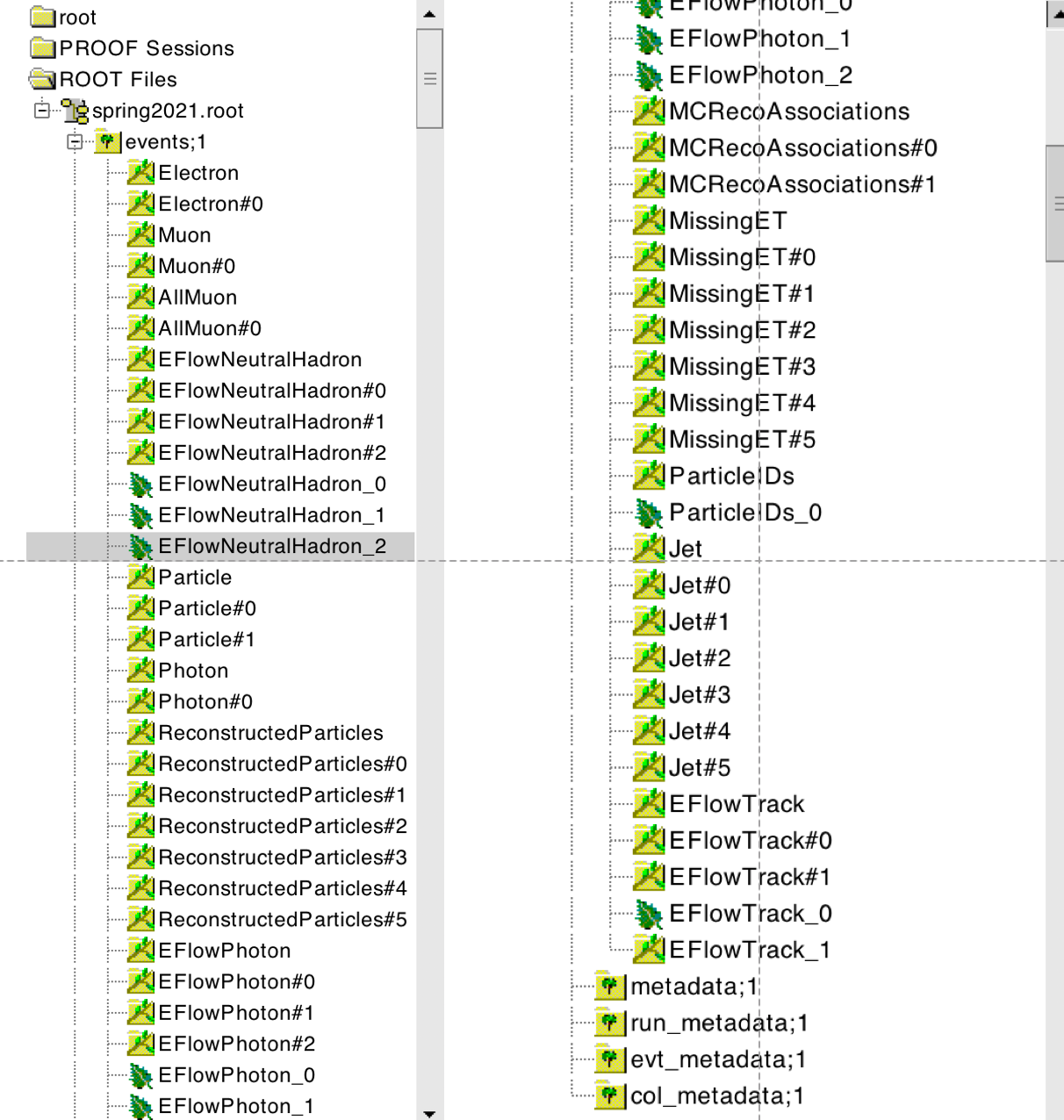
Example file from “spring2021” campaign in ROOT TBrowser.

As shown in the screenshot above, there are two types of branches:

1. Branches without a pound sign (#) in their name like: Electron, Muon, …
   They refer to collections of objects.

Nota Bene

Particle denotes the collection of Monte-Carlo particles. Muon contains the isolated muons, while AllMuon contains all muons, isolated or not.

2. Branches with a pound sign in their name:
   Each of the object collections listed above, e.g. Collection, has up to six associated collections of references, i.e. indices that point to another or to the same object collection. They are labeled Collection#i, with i = 0 ... 5. For example, the Muon collection has one single associated collection of references, Muon#0.

To figure out which collection is pointed to by Muon#0 (or by any other collection of references), one can look at the value of Muon#0.collectionID (see screenshot below). The collectionID of Muon#0 is the collection number 7 (in the example file used here), which, in the list of “object collections” above, corresponds to the collection of ReconstructedParticles. Indeed, the Muon collection itself contains nothing (see screenshot below): all the information is contained in the ReconstructedParticles. The Muon collection, together with Muon#0, just provides a convenient way to access, among the ReconstructedParticles, those that were identified as muons.

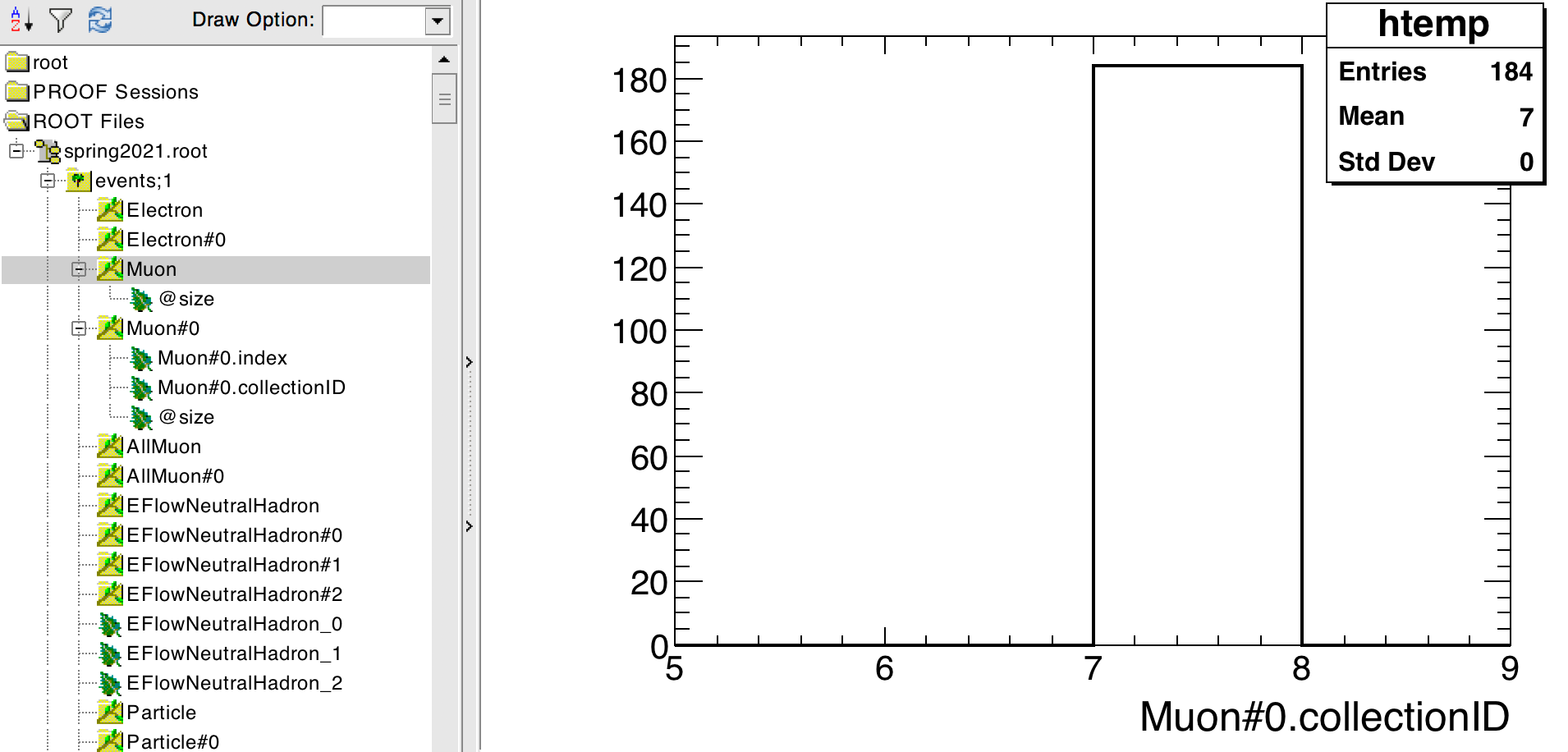
Muon collection example.

The same holds for the Electron and Photon collections. On the other hand, the MissingET collection is already a ReconstructedParticle, as can be seen by inspecting it in the TBrowser:

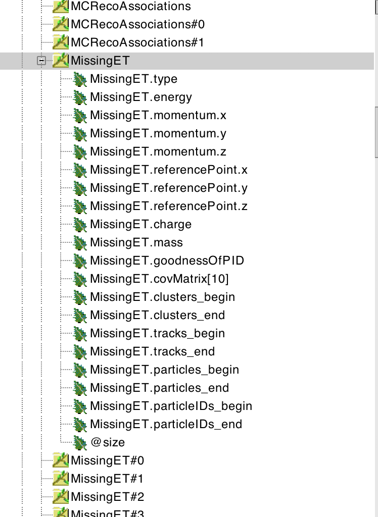
Missing \(E_T\) collection example.

The Particle collection corresponds to the Monte-Carlo particles. It has two associated collections of references, Particle#0 and Particle#1. As can be seen by looking at their collectionID, they both point to collection number 5, i.e. to the Particle collection itself. Particle#0 and Particle#1 contain, respectively, links to the parents and to the daughters of the MC particles — as can be seen in the EDM4hep yaml description here. Examples will be given below, showing how to navigate through the Monte-Carlo record using Particle, Particle#0 and Particle#1.

2.5.2. Overall organisation of analysis code (C++)

All the common code lives in FCCAnalyses namespace which is by default loaded when running fccanalysis command. Then each module of analyzers in one header file has its own dedicated namespace, thus to call a given function from a given module it should look like FCCAnalyses::<ModuleName>::<FunctionName> but <ModuleName>::<FunctionName> should also work. For example, to call get_px from the ReconstructedParticle module write: ReconstructedParticle::get_px(<BranchName>).

2.5.3. Reading objects from EDM4hep

The example read_EDM4HEP.py shows you how to access the different objects such as jets, electrons, muons, missing \(E_T\) etc. from the EDM4hep files. Generally a new variable is calculated with a statement inside the analysers(df) function of the RDFanalysis class like dataframe.Define("<your_variable>", "<accessor_fct (<name_object>)>") which creates a column in the RDataFrame named <your_variable> filled with the return value of the <accessor_fct> for the given object.

Here, accessor functions are the functions found in the C++ analyzers code that return a certain variable. Since the analyzers code defines a specific namespace for each module, such as ReconstructedParticle or MCParticle, the full accessor function call looks like <namespace>::<function_name>(object). To access the \(p_T\) of a reconstructed object you would therefore call ReconstructedParticle::get_pt(object) and for a MC-particle the call would be MCParticle::get_pt(object). The namespace corresponds to the file name of the C++ code, making it clear where to look for the source code if you have a question about the internal workings of one such functions.

Below you can find an overview of the basic, most commonly required functions, to illustrate the naming conventions. This is not an exhaustive list, if you want to find out all functions that are available please take a look in the respective analyzers code itself — here for reconstructed particles and here for MC particles.

Variable	Function name	Available for
Transverse momentum	get_pt(object)	MCParticle, ReconstructedParticle
Pseudorapidity	get_eta(object)	MCParticle, ReconstructedParticle
Energy	get_e(object)	MCParticle, ReconstructedParticle
Mass	get_mass(object)	MCParticle, ReconstructedParticle
Charge	get_charge(object)	MCParticle, ReconstructedParticle
Number (in event)	get_n(object)	MCParticle, ReconstructedParticle
PDG ID	get_pdg(object)	MCParticle

If you want to add your own function have a look at the Writing a new analyzer section on this page.

For the name of the object, in principle the names of the EDM4hep collections are used — photons, muons and electrons are an exception where a few extra steps are required, as shown in the example here.

This example also shows how to apply object selection cuts, for example selecting only reconstructed objects with a transverse momentum \(p_T\) larger than a given threshold by using the ReconstructedParticle::sel_pt(<threshold>)(<name_object>) function.

In the end of the example you can see how the selected variables are written to branches of the output n-tuple, using the dataframe.Snapshot("<tree_name>", <branch_list> ), where in all examples here the name of the output-tree is always events and the branch_list is defined as a ROOT.vector('string') as demonstrated in the example. Note that branches of variables that exist multiple times per event, i.e. anything derived from a collection such as the \(p_T\) of jets, result in vector branches. This is also true for some quantities that in principle only exist once per event, but are collections in the EDM4hep format, such as the missing transverse energy.

2.5.4. Association between RecoParticles and MonteCarloParticles

By design, the association between the reconstructed particles and the Monte-Carlo particles proceeds via the MCRecoAssociations collection, and its two associated collections of references, MCRecoAssociations#0 and MCRecoAssociations#1, all of the same size. The collectionID of MCRecoAssociations#0 is equal to 7 in the example file used here (see above, Structure of EDM4hep files), which means that MCRecoAssociations#0 points to the ReconstructedParticles. While the collectionID of MCRecoAssociations#1 is equal to 5, i.e. MCRecoAssociations#1 points to the Particle collection (i.e. the Monte-Carlo particles).

Their usage is best understood by looking into the code of ReconstructedParticle2MC::getRP2MC_index reported below:

ROOT::VecOps::RVec<int>
ReconstructedParticle2MC::getRP2MC_index(const ROOT::VecOps::RVec<int>& recind,
                                         const ROOT::VecOps::RVec<int>& mcind,
                                         const ROOT::VecOps::RVec<edm4hep::ReconstructedParticleData>& reco) {
  ROOT::VecOps::RVec<int> result;
  result.resize(reco.size(),-1.);
  for (size_t i=0; i<recind.size();i++) {
    result[recind.at(i)]=mcind.at(i);    // recind.at(i) is the index of a reco'ed particle in the ReconstructedParticles collection
                                         // mcind.at(i) is the index of its associated MC particle, in the Particle collection
  }

  return result;
}

which, in a FCCAnalyses configuration file, will be called via :

.Alias("MCRecoAssociations0", "MCRecoAssociations#0.index")
.Alias("MCRecoAssociations1", "MCRecoAssociations#1.index")
.Define('RP_MC_index',"ReconstructedParticle2MC::getRP2MC_index(MCRecoAssociations0, MCRecoAssociations1, ReconstructedParticles)")

(the first two Alias lines are needed for ROOT to understand the pound # sign).

The analyzer getRP2MC_index creates a vector that maps the reconstructed particles and the MC particles: RP_MC_index[ ireco ] = imc , where ireco is the index of a reco’ed particle in the ReconstructedParticle collection, and imc is the index, in the Particle collection, of its associated MC particle.

Careful

As can be seen from the code, the method getRP2MC_index must receive the full collection, ReconstructedParticles, and not a subset of reco’ed particles.

To retrieve the associated MC particle of one reco’ed particle, or of a subset of reco’ed particles, one should have kept track of the indices of these particles in the ReconstructedParticles collection. It can be a good practise to design analyses that primarily use indices of RecoParticles, instead of the RecoParticles themselves. However, for a charged reco’ed particle RecoPart, one can also use the following workaround:

int track_index = RecoPart.tracks_begin ;   // index in the Track array
int mc_index = ReconstructedParticle2MC::getTrack2MC_index(track_index, recind, mcind, reco);

where recind refers to MCRecoAssociations0, mcind to MCRecoAssociations1, and reco to ReconstructedParticles.

2.5.5. Navigation through the history of the MC particles

To retrieve the daughters of a Monte-Carlo particle (in the Particle collection), one should use the collection of references to daughters (Particle#1, which points to Particles), together with the Particle collection itself.

Each particle in the Particle collection contains two integers, daughters_begin and daughter_end. The indices, in the Particle collection, of the daughters of the particle are stored in Particle#1, between daughters_begin and daughter_end. This is illustrated in the code of MCParticle::get_list_of_daughters_from_decay (link) reported below:

std::vector<int>
MCParticle::get_list_of_particles_from_decay(int i,
                                             const ROOT::VecOps::RVec<edm4hep::MCParticleData>& in,
                                             const ROOT::VecOps::RVec<int>& ind) {

  std::vector<int> res;

  // i = index of a MC particle in the Particle block
  // in = the Particle collection
  // ind = the block with the indices for the daughters, Particle#1.index

  // returns a vector with the indices (in the Particle block) of the daughters of the particle i

  int db = in.at(i).daughters_begin ;
  int de = in.at(i).daughters_end;
  if  ( db == de ) return res;   // particle is stable
  for (int id = db; id < de; id++) {
     res.push_back( ind[id] ) ;
  }

  return res;
}

This returns the “first branching” daughters. For example, if we have a Higgs that decays into ZZ*, with both Z’s decaying into muons, the method get_list_of_daughters_from_decay, applied to i = the index of the Higgs, returns the indices of the two Z’s in the Particle collection. In order to retrieve the indices of the four muons, use instead MCParticle::get_list_of_stable_daughters_from_decay (link).

These functions are not meant to be called directly from the python configuration file, but from some other function that will determine the value of the argument i. See an example here in FCCeePhysicsPerformance, the important lines being:

.Alias("Particle1", "Particle#1.index")
# MC indices of the decay Bs -> Ds+ K-
# In the file I process, only the Bs0 (not the Bsbar) has been forced to decay into Ds+ K-
# Look for (Ds+ K-) in the list of unstable decays of a Bs - hence oscillations are
# not accounted for. So there should be at most one such decay per event. In any case,
# would there be > 1, the method gives the first one encountered.
# Returns the indices of : mother Bs, Ds+, K-

.Define("Bs2DsK_indices", "MCParticle::get_indices_ExclusiveDecay( -531, {431, -321}, false, false) ( Particle, Particle1)" )

Again, the first line is needed for RootDataFrame to interpret correctly the pound sign.

To retrieve the parents of a Monte-Carlo particle: the logic is the same, one should use parents_begin and parents_end, which point to the Particle#0 collection.

2.5.6. Writing a new analyzer

There are several ways how to define a new analyzer, which can have various forms and complexity. The analyzer then can be used in the RDF Define and Filter statements. Here we list several of them and their use cases, full RootDataFrame documentation can be viewed here.

2.5.6.1. C++ string

To define a simple analyzer one can use RDataFrame’s feature of providing functions directly as string of C++ code, something like:

.Define("myvec",
        "ROOT::VecOps::RVec<int> v; for (int i : { 1, 2, 3, 4, 5, 6, 7 }) v.push_back(i); return v;")
.Define("myvecsize", "myvec.size()")

2.5.6.2. Using ROOT gInterpreter

It is also possible to define more complex analyzer and feed it to the ROOT gInterpreter

ROOT.gInterpreter.Declare("""
template<typename T>
ROOT::VecOps::RVec<T> myRange(ROOT::VecOps::RVec<T>& vec, std::size_t begin, std::size_t end) {
  ROOT::VecOps::RVec<T> ret;
  ret.reserve(end - begin);
  for (auto i = begin; i < end; ++i)
    ret.push_back(vec[i]);
  return ret;
}
""")

and then call it in the Define

.Define("mysubvec", "myRange(myvec, 2, 4)")

2.5.6.3. Inside an existing FCCAnalyses module

When you believe you need to develop a new function within an existing FCCAnalyses namespace, you should proceed as follow:
In the corresponding header file in analyzers/dataframe/FCCAnalyses you should add the definition of your function, for example:

/// Get the invariant mass from a list of reconstructed particles
float getMass(const ROOT::VecOps::RVec<edm4hep::ReconstructedParticleData> & in);

In the corresponding source file in analyzers/dataframe/src you should add the implementation of your function, for example:

float getMass(const ROOT::VecOps::RVec<edm4hep::ReconstructedParticleData>& in) {
  ROOT::Math::LorentzVector<ROOT::Math::PxPyPzE4D<double>> result;

  for (auto & p: in) {
    ROOT::Math::LorentzVector<ROOT::Math::PxPyPzE4D<double>> tmp;
    tmp.SetPxPyPzE(p.momentum.x, p.momentum.y, p.momentum.z, p.energy);
    result+=tmp;
  }

  return result.M();
}

Note that for efficiency, the arguments should be passed as const reference.

If your code is simple enough, it can also add the function only to the header file and even templated, for example:

template<typename T>
inline ROOT::VecOps::RVec<ROOT::VecOps::RVec<T>> as_vector(const ROOT::VecOps::RVec<T>& in) {
  return ROOT::VecOps::RVec<ROOT::VecOps::RVec<T>>(1, in);
};

2.5.7. Writing a new struct

When you believe you need to develop a new struct within an existing namespace, you should proceed as follow: In the header file in analyzers/dataframe/FCCAnalyses you should add a struct or a class like:

/// Get the number of particles in a given hemisphere (defined by it's angle wrt to axis). Returns 3 values: total, charged, neutral multiplicity
struct getAxisN {
public:
  getAxisN(bool arg_pos=0);
  ROOT::VecOps::RVec<int> operator() (const ROOT::VecOps::RVec<float> & angle,
                                      const ROOT::VecOps::RVec<float> & charge);
private:
  bool _pos; /// Which hemisphere to select, false/0=cosTheta<0 true/1=cosTheta>0. Default=0
};

where the public members should contain the name of the function with the constructor arguments (in this example getAxisN) and the operator() that correspond to the function that will be evaluated for each event and return the output. The private section should contains members that will be needed at run time, usually the arguments of the constructor.

In the corresponding source file in analyzers/dataframe/src you should add the implementation of your class, for example:

getAxisN::getAxisN(bool arg_pos) {
  _pos=arg_pos;
}

ROOT::VecOps::RVec<int> getAxisN::operator() (const ROOT::VecOps::RVec<float> & angle,
                                              const ROOT::VecOps::RVec<float> & charge) {
  ROOT::VecOps::RVec<int> result = {0, 0, 0};

  for (size_t i = 0; i < angle.size(); ++i) {
    if (_pos==1 && angle[i]>0.){
      result[0]+=1;
      if (std::abs(charge[i])>0) result[1]+=1;
      else result[2]+=1;
    }
    if (_pos==0 && angle[i]<0.){
      result[0]+=1;
      if (std::abs(charge[i])>0) result[1]+=1;
      else result[2]+=1;
    }
  }

  return result;
}

where you separate the class construction and its implementation.

2.5.8. Writing a new module

If you think new module/namespace is needed, create a new header file in analyzers/dataframe/FCCAnalyses, for example MyModule. It should look like:

#ifndef  MYMODULE_ANALYZERS_H
#define  MYMODULE_ANALYZERS_H

// Add here your defines

namespace FCCAnalyses {
  namespace MyModule {

// Add here your analyzers
  }
}
#endif

create a new source file in analyzers/dataframe/src, for example myModule.cc. It should look like:

#include "FCCAnalyses/myNamespace.h"
// Add here your defines

namespace FCCAnalyses {
  namespace MyModule {
    // Add here your functions, structs

  }
}

2.5.9. Writing your own analysis using the case-studies generator

Experimental feature

The following feature is experimental and might not work as expected. Please, contact developers.

For various physics case studies, standard RDF tools might not be sufficient and require a backing library of helper objects and static functions exposed to ROOT.

An analysis package creation tool is developed to provide the minimal building blocks for such extensions and uniformise such developments.

2.5.9.1. Analysis package generation

Two modes are currently supported for the linking of these extensions to the analysis framework:

• scan at CMake+compilation time a standard extensions directory (in case-studies) where the analysis package can be deployed. It requires an includes and src subdirectory, along with a classes_def.xml and classes.h files in the latter for the ROOT dictionary definition.

• generate a standalone package which can be compiled independently, given the path to this FCCAnalyses installation is found. It allows to generate a minimal set of files required to connect this extension to the RDF utilitaries.

The generation of such a package can be done using the following recipe:

fccanalysis init [-h] [--name NAME] [--author AUTHOR] [--description DESCRIPTION] [--standalone] [--output-dir OUTPUT_DIR] package

where the mandatory parameter, package, refers to the analysis package name (along with the namespace it will define ; should be unique at runtime). Additionally, several optional parameters are handled:

• NAME specifies the analyser helpers filename (where all static functions exposed to the RDF framework through the ROOT dictionary will be stored) ;

• AUTHOR, preferably following the “name <email@address>” convention, and DESCRIPTION, will be added into the C++ files boilerplates to keep track of the author(s) and purpose(s) of this package ;

• --standalone to switch to the standalone package described above. In combination with the OUTPUT_DIR parameter, it allows to store the minimal working example in a completely arbitrary path (instead of the standard case-studies subdirectory) with its own CMake directive.

In the standalone mode, the analysis package can be built using the standard CMake recipe, given the FCCAnalyses environment in setup.sh is properly sourced:

mkdir build && cd build
cmake ${OUTPUT_DIR} && make
make install

The latter ensures that the headers and shared library/ROOT translation dictionaries are installed in a location reachable by FCCAnalyses.

2.5.9.2. Analysis package exposure to RDF

To allow an arbitrary multiplicity of analysis packages to be handled at the level of a configuration script runnable with “fccanalysis run”, an additional (optional) analysesList list-type object can be parsed.

On top of the usual FCCAnalyses shared object, includes, and corresponding dictionary, the custom case study analysis package name will be parsed, and automatically loaded in the ROOT runtime environment to be exposed to the RDF interface.