View on GitHub

FCCeePhysicsPerformance

General information

Common event samples
Example analyses and how-to’s
Code development
To produce your own Delphes samples
The five-parameter tracks produced by the Delphes interface
Vertexing and flavour tagging
Making particle combinations with awkward arrays
Generating events under realistic FCC-ee environment conditions
Monte-Carlo programs
Bibliography

Common event samples

(Oldish) The “spring2021” Monte-Carlo samples (May 2021)

some input on the MC production had been collected in early 2021 at this googledoc.
Details of the spring2021 samples:
- the production uses the EventProducer developed by C. Helsens.
- release from 2021-04-30, uses Delphes 3.4.3pre10
- configuration cards (delphes cards, Monte-Carlo cards): see the FCC-configs repository, branch spring2021. <!—
- Main changes compared to the “tmp” samples:
  - bugfix of the MC-associations for electrons
  - beam-pipe model updated
  - better resolution for displaced tracks;
  - the error matrix of the track parameters now include also the off-diagonal terms
  - addition of “inclusive” (non-isolated) muons in the output files –>
- See here for information about the files made with IDEA
- The event files can be found in EOS /eos/experiment/fcc/ee/generation/DelphesEvents/spring2021
- a few files were produced, corresponding to IDEA with a 3T field, and to “IDEA” where the Drift Chamber was repaced by the CLD tracker

Known caveats in the “spring2021” samples:

there is some inefficiency for electrons, due primarily to the overlap removal procedure, see Jean-Loup’s talk and here
the efficiency for very low momentum tracks is lower than what it should be, see Tristan’s talk and here
the jets that are on the EDM4Hep files, i.e. that were produced during the Delphes step, should not be used. See Jean-Loup’s talk and here. The issue lies in the Delphes card that was used (some jets are suppressed in the overlap removal procedure). The solution is to re-cluster the jets in FCCAnalyses, as explained below.

The “winter2023” Monte-Carlo samples (January 2023)

release from 2022-12-23, uses Delphes 3.5.1pre05
configuration cards (delphes cards, Monte-Carlo cards): see the FCC-configs repository, branch winter2023.
Main changes compared to spring2021 - see details here
- Updated IDEA geometry in the Delphes card:
  - smaller radius beam-pipe ( R = 1 cm )
  - ECAL crystal calorimeter hence much better ECAL resolution. Note that while the crystals are a seriously considered option, this is not yet the baseline of IDEA.
- Electrons and Muons are stored prior to any isolation requirement
- Track uncertainties are now reliable also for very displaced tracks
- fixed issues with electron inefficiencies and inefficiencies for low pT tracks. Overlap removal left to the user.
- Updated machine parameters (hence beam energy spread and size of the luminous region)
- Whizard samples now have a non-zero event vertex
- Jets that are on the files correspond to the ee_genkt algorithm, with p = -1 (i.e. antikT like), radius = 1.5, PTmin = 1 GeV. These jets may not be suited to all analyses, and as before, the best is to re-cluster the jets in FCCAnalyses, as explained below.
- Electron resolution: slightly degraded compared to muon resolution (by 20%), to account approximatively for the brems.
- Generator cards: Particles are decayed only if the decay vertex is within a cylindrical volume, corresponding to the volume of the tracker.
- The magnetic field is stored on the files (branch “magFieldBz”)
- For the tracks, the dNdx can be accessed in the “EFlowTrack_2” collection.
List of samples produced is here. More samples, esp. at 91 GeV, will be produced.
The event files can be found in EOS /eos/experiment/fcc/ee/generation/DelphesEvents/winter2023

Example analyses and how-to’s

Example analyses can be found in the FCCAnalyses repository. Checkout the master branch if you want to analyze EDM4HEP samples (the fccedm branch contains examples for the FCCSW-FCCEDM samples). And follow the instructions in the README of FCCAnalyses repository.

Basics

A first introduction to FCCAnalyses was also given in Clement’s talk at our December 2021 Phys Perf meeting.
Basic documentation can be found here. The configuration file read_EDM4HEP.py contains a few comments, which can help people get started.
First example, Higgs mass recoil : Simple example used in the README: examples/FCCee/higgs/mH-recoil/mumu/

How to associate RecoParticles with Monte-Carlo Particles

see explanations here <!—
see also the example in examples/FCCee/flavour/generic-analysis shows how the associations work (how to retrieve the Monte-Carlo particle associated to a reconstructed particle; how to retrieve the track of a reconstructed particle) –>

How to navigate through the history of the Monte-Carlo particles

see exaplanations here

How to compute event variables (thrust, sphericity, etc)

see an example in examples/FCCee/flavour/Bc2TauNu

How to fit tracks to a common vertex

To see how one can run the vertex fitter over a collection of tracks, see in examples/FCCee/vertex
see also the section devoted to vertexing in the software tutorial and some links below <!–
see also various examples in this repository, case-studies/flavour/VertexExamples –>

How to run jet algorithms

To see how one can run a jet algorithm over a collection of particles, see in examples/FCCee/top/hadronic. This is an interface to FastJet. See in JetClustering.h for more details and for the definition of the parameters.

The relevant lines in FCCAnalysis are given in the example below (here Durham algorithm, exclusive N=2) :

        # Jet clustering
       .Define("RP_px", "ReconstructedParticle::get_px(ReconstructedParticles) ")
       .Define("RP_py", "ReconstructedParticle::get_py(ReconstructedParticles) ")
       .Define("RP_pz", "ReconstructedParticle::get_pz(ReconstructedParticles) ")
       .Define("RP_e", "ReconstructedParticle::get_e(ReconstructedParticles) ")

       # build pseudo jets with the RP, using the interface that takes px,py,pz,E
       .Define( "pseudo_jets",  "JetClusteringUtils::set_pseudoJets(RP_px, RP_py, RP_pz, RP_e)" )

       # run jet clustering with all reconstructed particles. Durham algo, exclusive clustering N=2, E-scheme
       .Define( "FCCAnalysesJets_ee_genkt",  "JetClustering::clustering_ee_kt(2, 2, 1, 0)(pseudo_jets)" )
       .Define("jets_ee_genkt",  "JetClusteringUtils::get_pseudoJets( FCCAnalysesJets_ee_genkt )")
       # access the jets kinematics :
       .Define("jets_px",  "JetClusteringUtils::get_px( jets_ee_genkt )")
	    
       # access the jet constituents:
       .Define("jetconstituents_ee_genkt", "JetClusteringUtils::get_constituents(FCCAnalysesJets_ee_genkt) ")
		
   # access the "dmerge" distances:
   .Define("dmerge_23", "JetClusteringUtils::get_exclusive_dmerge( FCCAnalysesJets, 2)" )

You may want to remove e.g. leptons from the list of particles that are to be clustered by the jet algorithm. Example:

    .Define("my_recoparticles",  "ReconstructedParticle::remove( ReconstructedParticles,  my_leptons )")
    .Define("RP_px", "ReconstructedParticle::get_px( my_recoparticles ) ")
    etc..

remember: the jets that are on the (spring2021) EDM4Hep files should not be used, see the caveats above
details on the interface to FastJet in FCCAnalyses can be found in Julie Torndal’s thesis
please read the FastJet manual
Basic guidance on jet algorithms (& FastJet) at FCC-ee: talk by Gavin Salam, Gregory Soyez and Matteo Cacciari at the Physics Performance meeting of June 27, 2022. Most recommended.
Durham algorithm in exclusive mode is often a good choice. The “dmerge_{i, i+1}” distances (see the FastJet manual, and the snippet above) can then be used to disentangle i-jets like events from (i+1)-like events

How to run kinematic fits

see the ABCfit++ software package described in Julie Torndal’s thesis
stand-alone package for the while, see the github repo

Code development

Generalities:

Code that is “general”, expected to be useful for many analyses, is hosted into the FCCAnalyses repository.
Code that is very specific to an analysis is expected to go into the “case-studies” directory of the FCCeePhysicsPerformance repository. For example, in FCCeePhysicsPerformance/case-studies/flavour/dataframe/analyzers/, there is a Bs2DsK.cc which contains some code that is specific to the reconstruction of the Bs to DsK decay; for examples that use this code, and for the recipe to set up the envirionment, see in flavour/VertexExamples.
as a first step, since the setup is easier, you may start to develop some code (even if it is analysis-specific) locally, in your local FCCAnalysis, and move it later to FCCeePhysicsPerformance. Or, if your code is of general interest, make a pull request such that your code gets merged in the central FCCAnalysis repository.

How to add a new functionnality in FCCAnalysis:

all the code is in analyzers/dataframe
you may add a new function to an existing file, for example if you add some basic functionnality that works on the Monte-Carlo particles, like retrieving the MC particle with the highest energy, it makes sense to add it into MCParticle.cc
or you can create a new file MyStuff.cc (for example, FlavourTagging.cc, ParticleIdentification.cc, etc). In that case, you just need to create a MyStuff.h, a MyStuff.cc, and to add your MyStuff.h in the CMakeLists.txt file (look for the others .h)

To produce your own Delphes samples

Quick instructions for producing samples

(For FCCSW samples (old), see this part of the tutorial.)

For EDM4HEP samples, first define the environment :

source /cvmfs/fcc.cern.ch/sw/latest/setup.sh

and take the output configuration file, edm4hep_output_config.tcl from key4hep/k4SimDelphes/examples.

To run Pythia and Delphes :
```
DelphesPythia8_EDM4HEP $DELPHES_DIR/cards/delphes_card_IDEAtrkCov.tcl edm4hep_output_config.tcl your_pythia_card.cmd outputFile.root
```
Example cards for Pythia can be found here (not much populated yet), or in EOS at CERN, in /eos/fcc/ee/utils/pythiacards (which contains the cards for all the samples produced in November 2020).

To read an LHE input file and process it through Delphes: the executable is the same, DelphesPythia8_EDM4HEP, and your Pythia card should just contain:

! 3) Tell Pythia that LHEF input is used
Beams:frameType             = 4
Beams:setProductionScalesFromLHEF = off
Beams:LHEF = your_input_file.lhe    

To produce events with PYTHIA+EVTGEN and run them through Delphes:
```
DelphesPythia8EvtGen_EDM4HEP $DELPHES_DIR/cards/delphes_card_IDEAtrkCov.tcl edm4hep_output_config.tcl p8_ee_Zbb_ecm91_EvtGen.cmd evtgen.root DECAY.DEC evt.pdl Bu2D0Pi.dec 
```
where evtgen.root is your output event file; p8_ee_Zbb_ecm91_EvtGen.cmd can be picked up e.g. from /eos/fcc/ee/utils/pythiacards/p8_ee_Zbb_ecm91_EvtGen_Bu2D0Pi.cmd; Bu2D0Pi.dec is the EVTGEN file where you specify the exclusive decay(s) you want, see examples in the HEP-FCC/FCC-config repository; DECAY.DEC and evt.pdl are standard EVTGEN files that, with the environment as defined above, can be found in $EVTGEN.

Make simple changes to the tracker or beam-pipe description in Delphes

The geometry of the (central) beam-pipe and of the tracker is described in $DELPHES_DIR/cards/delphes_card_IDEAtrkCov.tcl for the IDEA tracker. (a version of this file, in which the IDEA drift chamber is replaced by the full-Si tracker of CLD, can be found in lxplus in /afs/cern.ch/user/s/selvaggi/public/4Emilia/delphes_card_CLDtrkCov_Tagging.tcl). To see the geometry description, look for the module TrackCovariance, and for the lines that are under set DetectorGeometry. The convention is as follows:

	// Layer type 1 = R (barrel) or 2 = z (forward/backward)
	// Layer label
	// Minimum dimension z for barrel  or R for forward  (m)
	// Maximum dimension z for barrel  or R for forward  (m)
	// R/z location of layera  (m)
	// Thickness (meters)
	// Radiation length of the material (in meters)
	// Number of measurements in layers (1D or 2D)
	// Stereo angle (rad) - 0(pi/2) = axial(z) layer - Upper side
	// Stereo angle (rad) - 0(pi/2) = axial(z) layer - Lower side
	// Resolution Upper side (meters) - 0 = no measurement
	// Resolution Lower side (meters) - 0 = no measurement
	// measurement flag = T, scattering only = F

For example, in the default description, the first line:

      1 PIPE -100 100 0.015 0.0012 0.35276 0 0 0 0 0 0

tells that the beam-pipe is at R = 1.5 cm (inner radius), has a thickness of 1.2 mm, and that the radiation length of the corresponding material is 0.35276 m (the X0 of Berrylium). In the next lines, corresponding to the vertex detector (barrel),

VTXLOW -0.12 0.12 0.017 0.00028 0.0937 2 0 1.5708 3e-006 3e-006 1
VTXLOW -0.16 0.16 0.023 0.00028 0.0937 2 0 1.5708 3e-006 3e-006 1
VTXLOW -0.16 0.16 0.031 0.00028 0.0937 2 0 1.5708 3e-006 3e-006 1

you see that the single hit resolution if each layer is 3 mum. At the end of this module, you see the value of the magnetic field that is used (set Bz 2.0), which also needs to be set in the ParticlePropagator module.

One can play with these values, to see e.g. how the performance changes when one sets the (beam-pipe and) innermost layer of the vertex detector closer to the beam-line, etc.

Change the Jet algorithm in the Delphes interface

The choice of which jet algorithm is run (for the jets that are written to the EDM4HEP file) is made in the Delphes cards. Note however that, at the analysis level, it is possible to re-run the jet clustering, using another algorithm than the one used when the file was produced. See above, “Example analyses”, for more information about this possibility. To change the algorithm that is run when the EDM4HEP file is produced, look up in the Delphes card:

module FastJetFinder GenJetFinder {
  set InputArray NeutrinoFilter/filteredParticles

  set OutputArray jets

  # algorithm: 1 CDFJetClu, 2 MidPoint, 3 SIScone, 4 kt, 5 Cambridge/Aachen, 6 antikt
  set JetAlgorithm 6
  set ParameterR 0.4
  set JetPTMin 1.0
}

In some cases, it may be desirable to run the algorithm in the “exclusive” mode, forcing the algorithm to produce a fixed number of jets. This can be done by setting the following parameters in the Delphes FastJet finder:

module FastJetFinder GenJetFinder {
   set ExclusiveClustering  True
   set NJets  2
.....
}

Algorithms that use the difference in (pseudo-)rapidity between particles in order to define the distance are not well suited for FCC-ee. At FCC, the center-of-mass of the collisions is at rest with respect to the detector, in contrast to what happens at pp colliders. And using Delta( Eta ), instead of Delta(theta) or Delta( cos theta) is harmful, since Delta( Eta ) is not a good measure of the angular separation: for two particles that are emitted close-by and at small angle, their difference in pseudo-rapidity diverges as the log of the polar angle. Hence, using a jet algorithm thar relies on Eta instead of the polar angle Theta will create too many jets in the forward region.
The VLC algorithm was largely used for CLIC studies (where it showed good performance in particular to reject the background from gamma gamma to hadrons, which is severe at CLIC).
See also the FastJet user manual

The five-parameter tracks produced by the Delphes interface

Recent versions of Delphes offer a rather detailed modelling of the tracks via the TrackCovariance Delphes module, developed from a code by Franco Bedeschi. The module, in the input card, must contain a description of the tracker, see for example the delphes_card_IDEAtrkCov.tcl. (more details about the geometry description can be found above). This produces five-parameter tracks - i.e., including the transverse and longitudinal impact parameters - with their covariance matrix.
- for more details about the TrackCovariance module, see Franco’s talk at the FCC detector meeting of March 2019, or at the CEPC meeting in Oxford, April 2019.

(old) In the FCCEDM output, the track parameters thar are saved are: ( d0, z0, phi, theta, q/p ) with d0 and z0 in mm and q/p in GeV-1 [TBC for q/p]. The covariance matrix is given in this basis. It is saved as 15 floats, trkCov[0], trkCov[5], trkCov[9], trkCov[12] and trkCov[14] denoting the diagonal elements of the symmetric matrix.
In the EDM4HEP output, the track parameters are (d0, phi, rho, z0, tanLambda), with d0 and z0 in mm and the curvature rho in mm^-1. The sign convention for the curvature rho is such that with Bz > 0 , rho is positive for a particle with Q > 0. The covariance matrix is saved as 15 floats corresponding to the former basis.
- For files produced before end of February 2021, only the diagonal elements of the covariance matrix of the track parameters were saved. And the matrix was saved as an upper-triangle matrix, trkCov[0], trkCov[5], trkCov[9], trkCov[12] and trkCov[14] denoting the diagonal elements of the symmetric matrix.
- Starting with the SW distribution deployed on Feb 26, 2021, the off-diagonal terms are stored too. Moreover, to comply with the convention used throughout EDM4HEP, it is now the lower-triangle matrix that is stored: trkCov[0], trkCov[2], trkCov[5], trkCov[9] and trkCov[14] denote the variances of d0, phi, rho, z0 and tanLambda; trkCov[1] is the covariance between d0 and phi, trkCov[3] between d0 and rho, etc.

Vertexing and flavour tagging

Topical meeting on vertexing, Feb 10, 2021

Link to the topical meeting on vertexing, Feb 10, 2021 organised jointly by Physics Performance and Software and Computing. And the meeting summary (plus progress) presented by Clement Helsens at the FCC-ee general meeting of February 22, 2021.

Informal e-group

An informal e-group was created after the topical meeting: vertexing-FCCee-informal

Vertex-fitter code from Franco Bedeschi

A stand-alone vertex-fitter from Franco Bedeschi has been implemented in FCCAnalyses.

the algorithm was described in Franco’s talk at the topical meeting on vertexing, Feb 10, 2021.
Franco presented an update at the Physics Performance meeting of July 18, 2022
In FCCAnalyses, see an example usage in examples/FCCee/vertex.
- analysis.py runs over Z to light jet events and determines the event primary vertex
- The macro vertex_plots.x makes plots of the chi2 of the fit, of the resolutions of the fitted vertex position in (x, y, z), and of the corresponding pulls.
- the code retrieves an edm4hep::VertexData object, where:
  - the vertex coordinates (x, y, z) are in mm
  - the returned chi2 is normalised to the number of degrees of freedom of the fit ( n.d.f. = 2 x N_tracks -3)
  - the covariance matrix of (x, y, z) is stored as a an array of 6 floats, corresponding to the lower-triangle matrix (i.e. covMat[0], covMat[2], covMat[5] denote the variances of x, y, z, respectively)
- the code is in analyzers/dataframe/VertexFitterSimple.cc, and makes use of analyzers/dataframe/VertexingUtils.cc
Examples that run this vertex fitter and determine resolutions of displaced vertices, in example exclusive B decay processes, can be found in the FCCeePhysicsPerformance repository, in case-studies/flavour/VertexExamples vertex resolutions
- with configuration files (analysis_xxx.py) and plotting macros (plots_xxx) that run over the ntuples created by the configuration files, and produce plots like those shown in Clement’s and Emmanuel’s talk at the topical meeting

Vertexing with the ACTS suite

see the talks of Andrea Salzbuger and of Bastian Schlag at the topical meeting of Feb 2021, for an overview of the ACTS project and a report on the ACTS vertexing suite
The ACTS vertexing suite is interfaced with FCCAnalyses.
- see example usage in examples/FCCee/vertex/analysis.py to see how one can run the AMVF vertex finder and the Billoir vretex fitter
- the code is in analyzers/dataframe/VertexFinderActs.cc and analyzers/dataframe/VertexFitterActs.cc
- same convention as described above for the quantities that are retrieved

The LCFIPlus algorithm

The LCFIPlus algorithm, developed for ILC and CLIC and used in the CLD performance paper.

Description of the LCFIPlus algorithm T. Suehara,T. Tanabe, arXiv1506.08371
LCFIPlus in GitHub
Talk from Clement Helsens, Oct 19, 2020
- the algorithm was run on EDM4HEP samples using a converter to LCIO as a first step.
the status of the implementation into key4hep as reported at the topical meeting of Feb 10, 2021 (P. Fernandez, A. Sailer)
Implementation in FCCAnalyses, talk from K. Gautam, A. Ilg and E. Ploerer, May 16, 2022

The DecayTreeFitter (DTF) algorithm

The DecayTreeFitter algorithm was developed at BaBar and is used at BaBar, LHCb and Belle-2.

Decay Chain Fitting with a Kalman Filter W. D. Hulsbergen, Nucl.Instrum.Meth.A 552 (2005) 566
Global Decay Chain Vertex Fitting at B-Factories J.-F. Krohn et al, NIM A, Volume 976, 2020, 164269: the implementation of Belle-II
the overview talk from Wouter Hulsbergen at the topical meeting of Feb 10, 2021
the LHCb gitlab repository

Flavour tagging using machine learning

see the work done in the context of the Hcc case study
status report: see the talk of K. Gautam at the FCC week, June 2022

Making particle combinations with awkward arrays

Combinatoric functions provided by the python awkward array pckage are very helpful to make particle combinations - e.g. loop over all Kaons and pions to find D candidates. To use them, the files should be analyzed with uproot. Very nice examples of how to use uproot and awkward arrays have been prepared by Donal Hill, see this repository.

see also Donal’s talk, Sep 21, 2020
the the scikit-hep software project

Generating events under realistic FCC-ee environment conditions

Beam energy spread

At FCC, the energy of the beams is distributed according to a Gaussian function. The corresponding beam energy spread is given in Table S.1 of the CDR, see the highlighted line here - these parameters were used for the spring2021 samples - or in the December 2022 parameters table, used for the winter2023 samples. One should use the second number, the one that corresponds to “BS” (with beamstrahlung). For example, at the Z peak, the beam energy spread amounts to 0.132%. Note that this is the spread of the energy of the beam; to get the relative spread of the centre-of-mass energy √s, these numbers have to be divided by √2.

It is important to take into account the beam energy spread when generating events. Some Monte-Carlo programs (e.g. Whizard) offer a built-in possibility to convolute the matrix elements with a Gaussian beam energy distribution.

For example, with Whizard, at √s = 240 GeV where the beam energy spread amounts to 0.185% (Dec 2022 parameters), the steering card should contain:

beams = e1, E1 => gaussian => isr
gaussian_spread1 = 0.185%
gaussian_spread2 = 0.185%

Vertex distribution

Bunch dimensions:
- The bunch length is given by the σ_z line in the CDR table (used for the spring2021 samples) or in the December 2022 table (used for the winter2023 samples); one should use the second number, corresponding to the “BS” (with beamstrahlung case). For example, at the Z peak, it amounts to 12.1 mm with the CDR parameters, and to 15.4 mm with the Dec 2022 parameters.
- The bunch dimensions in the transverse plane, at the interaction point, are given by σ_x,y = √ ( β*_x,y ε_x,y) where the values of the β function at the IP, and the horizontal and vertical emittance ε_x,y are given in the CDR table or in the December 2022 table.
For gaussian bunches, the vertex distribution in (x, y, z) and in time is well approximated by a 4-dimensional gaussian distribution, with (see here ): 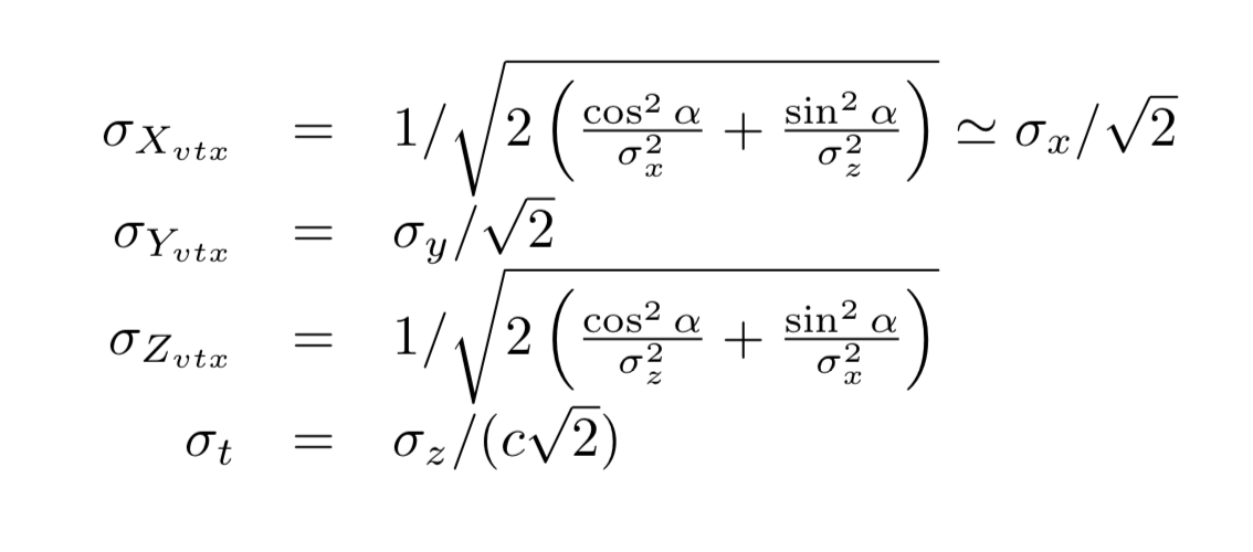where α denotes the half-crossing angle, α = 15 mrad.

Summary table, CDR parameters :

Ebeam (GeV)	45.6	80	120	175	182.5
σ_x (µm)	6.4	13.0	13.7	36.6	38.2
σ_y (nm)	28.3	41.2	36.1	65.7	68.1
σ_z (mm)	12.1	6.0	5.3	2.62	2.54
Vertex σ_x (µm)	4.5	9.2	9.7	25.9	27.0
Vertex σ_y (nm)	20	29.2	25.5	46.5	48.2
Vertex σ_z (mm)	0.30	0.60	0.64	1.26	1.27
Vertex σ_t (ps)	28.6	14.1	12.5	6.2	6.0

Summary table, December 2022 parameters:

Ebeam (GeV)	45.6	80	120	182.5
σ_x (µm)	8.4	20.8	13.9	38.6
σ_y (nm)	33.7	65.7	35.9	69.1
σ_z (mm)	15.4	8.0	6.0	2.74
Vertex σ_x (µm)	5.96	14.7	9.8	27.3
Vertex σ_y (nm)	23.8	46.5	25.4	48.8
Vertex σ_z (mm)	0.397	0.97	0.65	1.33
Vertex σ_t (ps)	36.3	18.9	14.1	6.5

Transverse boost to account for the crossing angle

Monte-Carlo programs generate events in a frame where the incoming particles collide head-on. The crossing angle in the (x, z) plane results in a transverse boost along the x direction. The parameter of the Lorentz transformation is given by : γ = √ ( 1 + tan² α ), where α denotes the half-crossing angle, α = 15 mrad. Hence, prior to be sent to the detector simulation, the 4-vectors of the particles in the final state have to be boosted according to :

drawing

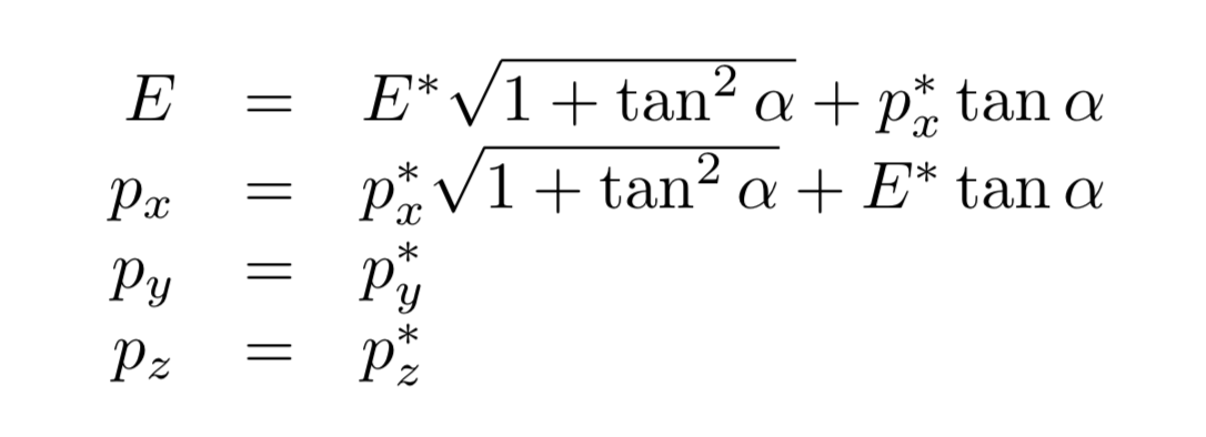
where the “star” quantities denote the kinematics in the head-on frame, and the quantities on the leftside of the formulae correspond to the kinematics in the detector frame.

The convention used here is that the incoming bunches have a positive velocity along the x axis. It is this convention that is used in the DD4HEP files that model the interaction region (i.e. the center of the LumiCals is at x > 0).

Monte-Carlo programs

Tutorial for Whizard for e+e- (Sep 2020)
- the Whizard main page with the online manual
KKMC : the state-of-the-art Monte Carlo for e−e+ → ffbar + nγ
- KKMC-ee in GitHub
- Talk by Martin Chrzaszcz, Oct 19, 2020

Bibliography

The CLD performance paper on arXiv N. Bacchetta et al,arXiv:1911.12230
Physics and Detectors at CLIC: CLIC Conceptual Design Report The CLIC Physics CDR, L.Linssen et al
The CEPC CDR, Physics and Detector CEPC study group, arXiv:1811.10545
The ILC TDR : Physics and Detectors